
Aktienbewegungen können als Zufallsprozess verstanden werden:
Der Aktienkurs 𝑆(𝑡) zum Zeitpunkt 𝑡 gemäß der geometrischen Brown’schen Bewegung ist gegeben durch:
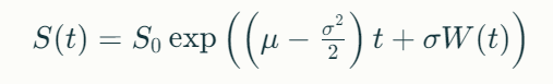
Dabei ist:
- 𝑆0 der Anfangsaktienkurs
- 𝜇 der Driftkoeffizient (erwartete Rendite)
- 𝜎 die Volatilität (Standardabweichung der Renditen)
- 𝑊(𝑡) ein Wiener-Prozess (standardisierte Brownsche Bewegung)
Solche Zufallsprozesse können simuliert werden:

Der Python-Code für diesen Prozess ist unten gegeben. Wer kein Python hat, kann einfach online (https://www.mycompiler.io/de/new/python) diesen Code kopieren und dann Ausführen lassen.
import numpy as np
import matplotlib.pyplot as plt

def geometric_brownian_motion(S0, mu, sigma, T, N):
    """
    Simulate a geometric Brownian motion.

    Parameters:
    S0 (float): Initial stock price
    mu (float): Drift coefficient (percentage)
    sigma (float): Volatility (percentage)
    T (float): Total time in years
    N (int): Number of time steps

    Returns:
    tuple: Time array and stock price array
    """
    dt = T / N
    t = np.linspace(0, T, N)
    W = np.random.standard_normal(size=N)
    W = np.cumsum(W) * np.sqrt(dt)  # Brownian motion
    X = (mu - 0.5 * sigma**2) * t + sigma * W
    S = S0 * np.exp(X)  # Geometric Brownian motion
    return t, S

def exponential_curve(S0, mu, T, N):
    """
    Calculate the exponential curve with the same drift.

    Parameters:
    S0 (float): Initial stock price
    mu (float): Drift coefficient (percentage)
    T (float): Total time in years
    N (int): Number of time steps

    Returns:
    tuple: Time array and exponential curve values
    """
    t = np.linspace(0, T, N)
    exp_curve = S0 * np.exp(mu * t)
    return t, exp_curve

# Set parameters
S0 = 100  # Initial stock price
mu = 0.1  # Drift (10% per year)
sigma = 0.15  # Volatility (15% per year)
T = 9000 / 365  # Total time in years (740 days)
N = 740  # Number of time steps (daily)

# Generate geometric Brownian motion
t, S   = geometric_brownian_motion(S0, mu, sigma, T, N)
t2, S2 = geometric_brownian_motion(S0, mu, sigma, T, N)

# Calculate the exponential curve
t_exp, exp_curve = exponential_curve(S0, mu, T, N)

# Plotting
plt.figure(figsize=(12, 6))
plt.plot(t, S, label='Geometric Brownian Motion')
plt.plot(t2, S2, label='Geometric Brownian Motion 2')

plt.plot(t_exp, exp_curve, label='Exponential Curve', linestyle='--')
plt.xlabel('Time (years)')
plt.ylabel('Stock Price')
plt.title('Geometric Brownian Motion vs Exponential Curve')
plt.legend()
plt.grid(True)
plt.show()